Part 1: The Ahmed Miscibility Function
Every CO₂ EOR project depends on the minimum miscibility pressure.
Above the MMP, CO₂ and oil become miscible — interfacial tension vanishes, residual oil drops sharply, and recovery improves significantly. Below it, the fluids remain as separate phases and sweep efficiency suffers.
In a recent project I helped evaluate CO₂ injection potential in a giant Middle East carbonate reservoir. The fluid data remain confidential. The workflow can be reproduced using public data.
This two-part series does exactly that — using open-source Python and published slimtube experiments to calculate CO₂ MMP and compare analytical predictions against laboratory measurements and compositional simulation.
Objectives
- Implement Ahmed's (1994) EOS-based miscibility function in Python and verify it against two published slimtube datasets.
- Build and run an E300 compositional slimtube simulation on the same fluids and compare the result against both the analytical method and the physical experiment.
- Establish a complete, reproducible CO₂ MMP screening workflow that any engineer can run without a commercial PVT package.
Part 1 covers the analytical method. Part 2 covers the E300 simulation. All code is available on GitHub.
Results First
| Fluid | Temperature | Slimtube exp. | Ahmed (2000) | This work | Error |
|---|---|---|---|---|---|
| A | 109°F | ~1500 psia | 1493 psia | 1549 psia | +3.3% |
| B | 103°F | ~2015 psia | 1999 psia | 2013 psia | −0.1% |
Both fluids are from Rathmell, Stalkup and Hassinger (1971) SPE 3483 — one of the few published datasets that releases full fluid compositions, EOS parameters, and slimtube results together. Ahmed used the same fluids to validate his method in CIPC 2000-01, giving a genuine three-way comparison: physical experiment, Ahmed's published prediction, and this Python implementation.
The Fluid A overprediction is real but bounded. Rathmell's data bracket the MMP between 1200 psig (immiscible) and 1500 psig (miscible), so 1549 psia sits just outside the experimental window. For Fluid B, where the long-core data are conclusive at 2000–2015 psig, the 2013 psia prediction is excellent.
EOS Setup
The fluids were characterised using a Peng–Robinson EOS with Peneloux volume correction. Standard EOS parameters were generated from critical properties and acentric factors, with C7+ critical temperature regressed against the experimental bubble point in PVTi 2023.1. The Python implementation reproduces the PVT package bubble point within 0.1% for both fluids.
Ahmed's contribution is surprisingly simple. He made two modifications to standard PR:
1. Fix αCO₂ = 1. Standard PR uses a temperature-dependent alpha function calibrated to CO₂ vapour pressure below its critical temperature of 88°F. Above this temperature — which covers essentially all reservoir conditions — the standard function extrapolates poorly, underestimating CO₂ density and producing optimistic MMP predictions. Setting αCO₂ = 1 and recalibrating the attraction and co-volume parameters against Vukalvich and Altunin's (1968) CO₂ density data corrects this. At 103°F, the modified parameters give CO₂ density approximately 8% higher than standard PR.
2. Revised CO₂–hydrocarbon BIPs. Standard BIPs between CO₂ and hydrocarbons default to 0.10 — reasonable, but not calibrated for miscibility prediction. Ahmed optimised these against slimtube data:
Each modification independently increases the predicted MMP:
| BIP configuration | Fluid B MMP (psia) | vs experimental 2015 psia |
|---|---|---|
| Standard (0.10 flat) | 1887 | −6.4% |
| Ahmed HC only | 1936 | −3.9% |
| Ahmed C7+ only | 1957 | −2.9% |
| Ahmed full | 2013 | −0.1% |
Everything else is standard PR EOS machinery.
The Ahmed Miscibility Function
The workflow follows five steps:
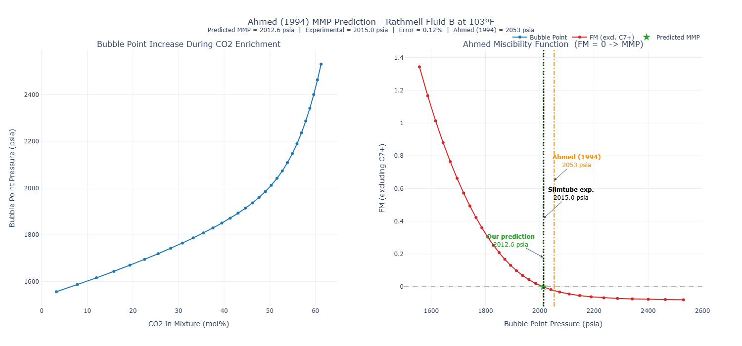
As CO₂ is added incrementally to the oil, the bubble point of the enriched mixture rises. K-values at the bubble point measure how far each component is from the critical condition where Ki = 1 for all components simultaneously. Ahmed's miscibility function (equation 19, SPE 27032) quantifies that distance:
At low CO₂ fractions, K-values are far from unity and FM is large and positive. As CO₂ content increases and pressure rises, K-values converge toward unity and FM approaches zero. The bubble point pressure at which FM = 0 is the MMP.
The parallel with the physical slimtube is direct: the slimtube finds miscibility through recovery vs pressure; the FM function finds it through K-value convergence vs pressure. Both identify the same condition — the pressure at which the CO₂–oil system reaches its critical point.
The C7+ Exclusion
With a single lumped C7+ pseudocomponent, KC7+ at bubble point conditions is of order 10⁻⁵ — five orders of magnitude below unity. Including this term drives FM to order 10,000 and the function never approaches zero at any achievable pressure.
Vaporising-gas-drive miscibility is controlled by intermediate hydrocarbons (C₂–C₆), not heavy ends. CO₂ extracts the intermediates into the vapour phase; the C7+ fraction remains in the liquid throughout. Excluding components with K < 10⁻⁴ from the FM sum is physically justified and produces monotonically decreasing FM curves with a well-defined zero crossing.
Results
Fluid A — T = 109°F. The FM curve decreases smoothly from approximately 0.85 at zero CO₂ addition to zero at 1549 psia. The zero crossing is sharp and well-defined. Rathmell's data bracket the MMP between 1200 psig (immiscible) and 1500 psig (miscible). The prediction of 1549 psia sits just above the upper bound, consistent with the known behaviour of the method at lower temperatures and lighter C7+ fractions.
Fluid B — T = 103°F. The FM curve reaches zero at 2013 psia and is within Rathmell's long-core experimental range of 2000–2015 psig.
Full Python implementation and notebook: github.com/eskoantg/CO2_MPP
Caveats
Ahmed's method answers one question: at what pressure does the CO₂–oil system reach its critical point under equilibrium conditions? Three things it does not capture:
Numerical dispersion. In a finite-difference simulator, grid blocks mix fluids over finite volumes, spreading the transition zone and delaying the development of a miscible front. A 100-cell slimtube model may predict a different MMP than a 1500-cell model of the same system. The Ahmed function has no grid — it is inherently dispersion-free.
The recovery curve shape. Ahmed's method gives a single pressure. The slimtube gives a full recovery curve — the rising slope below MMP, the kink at MMP, the plateau above it. The shape of this curve contains information about how readily miscibility develops in a real reservoir. Part 2 addresses this directly.
Drive mechanism competition. For fluids where both condensing and vaporising mechanisms contribute, the pure vaporising assumption may not hold. Both Rathmell fluids are unambiguously vaporising — confirmed by the FCMP composition (78.6 mol% CO₂ at 6908 psia for Fluid B) and a ratio FCMP/MCMP ≈ 3.4 consistent with a vaporising drive system. For other fluids, caution is warranted.
- The E300 slimtube model — matched to the same lab geometry as the Rathmell experiments, five pressures spanning 1600–2300 psia.
- Recovery at 1.2 pore volumes injected plotted against pressure. The Horner extrapolation to zero-dispersion recovery and why it is essential.
- How close does a compositional finite-difference simulation get to the physical experiment and to the Ahmed analytical estimate? And what does the simulation tell us that the analytical method cannot?
Rathmell, J.J., Stalkup, F.I. and Hassinger, R.C. (1971). A Laboratory Investigation of Miscible Displacement by Carbon Dioxide. SPE 3483.
Ahmed, T.H. (1994). Prediction of CO₂ Minimum Miscibility Pressures. SPE 27032.
Ahmed, T.H. (2000). Minimum Miscibility Pressure from EOS. CIPC Paper 2000-01.
Yellig, W.F. and Metcalfe, R.S. (1980). Determination and Prediction of CO₂ Minimum Miscibility Pressures. JPT, January 1980.
Peng, D.Y. and Robinson, D.B. (1976). A New Two-Constant Equation of State. Ind. Eng. Chem. Fundamentals, 15(1).
Peneloux, A., Rauzy, E. and Freze, R. (1982). A Consistent Correction for Redlich-Kwong-Soave Volumes. Fluid Phase Equilibria, 8(1).
Vukalvich, M.P. and Altunin, V.V. (1968). Thermophysical Properties of Carbon Dioxide. Collet's Ltd., London.