Screening Injection Support with the Energy Method

16 Jun 2026

Before running a complex method to quantify well connectivity like CRM, there is a simpler question to answer: is there any evidence that an injector and producer are connected in the first place?

On a field with one producer and two injectors that question is trivial. On a mature waterflood with dozens of wells, running CRM on every possible injector-producer pair is time-consuming and most combinations may contain little more than noise. A fast screening step helps focus the effort.

The Energy Method is that screening step. It does not quantify connectivity. It provides an indication of whether two rate signals are coherent enough to suggest a real reservoir connection.

This post shows how the Energy Method was applied to producer F-14 at Volve before the CRM analysis discussed in the previous post.

Why F-14

F-14 is one of two wells that carried the Volve field. Together with F-12 it accounted for roughly 86% of total field production. F-12 produced 4.6 MSm³ of oil, F-14 produced 3.9 MSm³. The three infill wells drilled in 2013–2014 (F-11, F-1 C, F-15 D) started with low watercut, but never approached those rates.

F-14 was the obvious candidate for a connectivity study. Two injectors support it: F-4 to the south and F-5 to the east, both roughly 1 km from the producer's reservoir entry point.

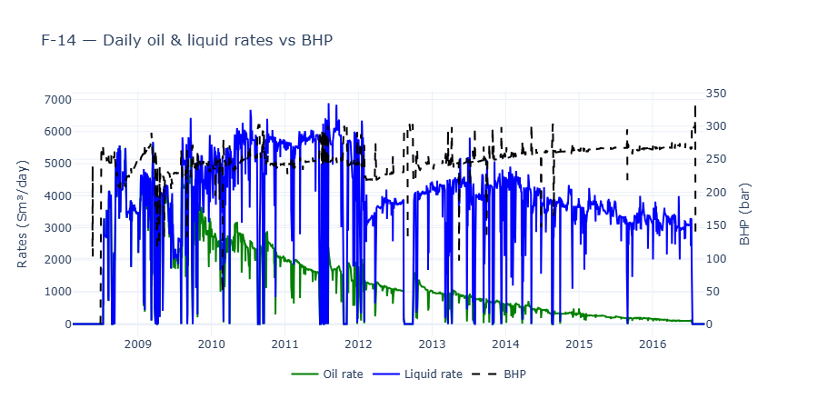
Figure 1: Well F-14 — Production Performance

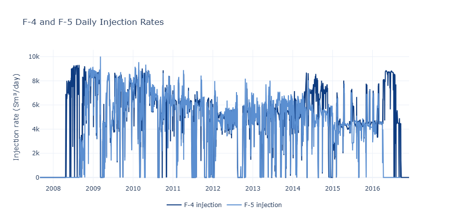
Figure 2: Injectors F-4 and F-5 — Injection Performance

The Method

The Energy Method applies the Teager-Kaiser Energy Operator (TKEO) to production and injection rate time series. The operator captures how much a signal is changing at each point in time:

\[ \Psi[x(n)] = x(n)^2 - x(n+1) \cdot x(n-1) \]

A flat rate produces almost no TKEO signal. A sudden rate change, shutdown, or operational adjustment produces a strong response. The method is designed to pick up activity in the signal rather than its absolute level.

For two signals x (injection) and y (production), a cross-energy version measures whether they fluctuate together:

\[ \Psi_B[x,y](n) = x(n) \cdot y(n) - x(n+1) \cdot y(n-1) \]

SimilB normalises the cross-energy into a score between 0 and 1:

\[ \text{SimilB} = \frac{\sqrt{2}\,\left|\displaystyle\sum \Psi_B(x,y)\right|}{\displaystyle\sum \sqrt{\Psi_B^2(x,x) + \Psi_B^2(y,y)}} \]

Computed over a rolling 30-day window on daily rate data, it produces a track over time: how coherent are these two signals right now, and does that coherence change.

A score near 1 indicates strong coherence between the two signals, while a score near 0 suggests they are behaving independently. Real field data are noisy, so connected wells typically score well below 1. Comparison against synthetic unconnected pairs confirmed that both injectors sit comfortably above the noise floor.

One important caveat: TKEO amplifies change, not level. A steady injector supporting a steadily declining producer will show near-zero SimilB even if the connection is strong. The method is only useful when both signals have coherent fluctuations within the rolling window. On Volve there is enough operational variability in the data for the method to work.

Result

EM was run in two configurations.

Rate-based: injection rate versus F-14 liquid rate. Both injectors peak at 0.41–0.42, with F-5 coming out slightly stronger than F-4. Both sit comfortably above the noise floor throughout most of the field life.

BHP-based: injection rate versus F-14 monthly mean downhole pressure. This is closer to how Ezabadi et al. (2023) applied the method using PDG data in a complex multi-stack reservoir. The BHP signal is a more direct reservoir response — it picks up the pressure pulse from the injector before it reaches the surface as a measurable rate change.

Figure 3: SimilB coherence score — F-4 and F-5 vs F-14 (rate-based and BHP-based)

Both F-4 and F-5 show coherent signal with F-14 above the noise floor. This is enough to proceed with CRM to quantify connectivity.

What the Energy Method was not intended to tell in this exercise:

How much of F-14's production each injector supports
The response time between injection and production
Whether the remaining ~25% of production support comes from the aquifer

Such questions can be addressed with more complex methods.

What the Screen Found

The Energy Method took five minutes to run and answered three questions before CRM was fitted:

Is F-4 connected to F-14? Yes
Is F-5 connected to F-14? Yes
Which is stronger? F-5, marginally

The workflow is straightforward: EM first, CRM second. EM identifies the likely connections. CRM quantifies them.

To reproduce the method, the code is on GitHub.

References

Kaiser, J.F. (1990). On a simple algorithm to calculate the 'energy' of a signal. IEEE ICASSP.

Baker, R., Sandhu, K., Radovic, P. and Saks, D. (2011). Characterization of Waterflood Communication. GOXC11-119.

Ezabadi, M.G. et al. (2023). Production Data Analysis of Smart Well Completion Revealed the Unknowns of Water Injection in a Heavily Faulted Multi-Stacked Reservoir. SPE-216181-MS.

Volve data licensed by Equinor under the Volve Data Village licence.