EOS Regression in Python: Closing the Gap to Lab Bubble Point
Part 1 and Part 2 established the full PR3 EOS engine — characterisation from MW and SG, mixing rules, cubic solver, fugacity coefficients, and bubble point pressure — all verified against commercial software exactly. The untuned result was 200.84 bar at 107°C. The lab measured 213.1 bar. This post closes that gap.
The Available Data
The laboratory dataset for this fluid contains a Constant Composition Expansion (CCE) experiment. The bubble point is identified directly from the discontinuity in the pressure-volume relationship — the point where the fluid transitions from single-phase liquid to two-phase. No Differential Liberation (DL) experiment was performed, meaning there are no GOR, Bo, or multi-pressure density observations available.
This gives a single reliable observation:
What Regression Does
The untuned EOS uses default Kesler-Lee critical properties throughout. These are deterministic outputs of the characterisation correlations. They are not fitted to any experimental data. The gap between 200.84 bar and 213.1 bar reflects the inherent uncertainty in estimating pseudocomponent properties from MW and SG alone.
Regression adjusts EOS parameters to minimise the difference between calculated and observed values. The objective function here is simply:
The parameters available for adjustment are the critical properties of the pseudocomponents — Tc, Pc, ω for C7-C15 and C16+. Standard practice is to start with the minimum number of variables and add more only if needed.
Variable Selection
With one observation (Pb) and the goal of minimum regression variables, the starting point is Tc,C16+ only.
C16+ dominates the mixture. At 15.9 mol% with ai = 1.49×10⁹ cm⁶·bar/mol² — 850 times larger than C1 — it controls Amix more than any other component. Increasing Tc,C16+ raises α, raises ai, raises Amix, and therefore raises the bubble point. It is the highest-leverage single variable.
Monotonicity constraint:
The upper bound of 1400 K is a physical limit. Beyond this the critical properties become unrealistic for any petroleum fraction.
Regression Implementation
The structure has three nested loops:
- Outer loop — scalar minimisation over Tc,C16+ using Brent's method (scipy minimize_scalar)
- Middle loop — bubble point pressure solver using Brent's method on the pressure axis
- Inner loop — successive substitution for K-value convergence at each trial pressure
The objective is evaluated by running the complete bubble point calculation at each trial Tc,C16+ value. No gradients are required. With one variable and one observation the problem is exactly determined and any convergent method finds the same answer.
Result
| Tc,C16+ (K) | Pbub (bar) | Δ from target |
|---|---|---|
| 993.22 (untuned) | 200.84 | −12.26 |
| 1020 | 206.41 | −6.69 |
| 1050 | 212.69 | −0.41 |
| 1080 | 219.02 | +5.92 |
| 1100 | 223.26 | +10.16 |
| 1200 | 244.95 | +31.85 |
The sensitivity is approximately 1 bar per 5 K increase in Tc,C16+. The target sits between 1050 and 1080 K — well within physical range.
| Value | |
|---|---|
| Tc,C16+ untuned | 993.22 K |
| Tc,C16+ tuned | 1051.97 K |
| Change | +58.75 K (+5.92%) |
| Pbub untuned | 200.84 bar |
| Pbub tuned | 213.10 bar |
| Target | 213.10 bar |
| Δ | 0.000 bar |
The tuned Tc,C16+ = 1051.97 K is consistent with the commercial software regression output for this fluid. This confirms the Python implementation reproduces not only the untuned EOS but the full regression workflow.
What the Tuned EOS Represents
The tuned Tc,C16+ = 1051.97 K is not a physical property of the C16+ fraction. It is an effective parameter. Its value compensates for all the modelling assumptions in place: the two-pseudo split of C7+, the Kesler-Lee correlations, the Katz-Firoozabadi BIPs and the PR3 formulation.
This is the nature of EOS regression in general. Parameters are adjusted within physically reasonable bounds to match observed data. The result is a tuned model valid for interpolation within the conditions of the matched experiment.
Standard practice is explicit on this: regression should use the minimum number of variables, preserve monotonicity of critical properties, and be validated against all available observations before use in simulation.
With only CCE data available, the tuned model is validated against one point. For a production-quality simulation model, differential liberation, separator tests and density measurements would extend the validation range and potentially require additional regression variables.
Closing Thoughts
This series reproduced the full PVT workflow — characterisation, EOS engine, and regression — from first principles in Python, matching every result exactly.
The core thermodynamic engine used in commercial PVT software was developed by specialist teams in the late 1980s and early 1990s — before numpy, before scipy, before any of the computational infrastructure we now take for granted. What that work took years to build, an engineer with Python can now reproduce in days. Not replace — the commercial tools carry decades of validation, edge case handling, and integration with simulation workflows. But understand, verify, and implement independently — that is now accessible in a way it simply was not before.
The engineer who understands what sits inside the software makes better decisions. They know which parameters to regress and why. They recognise when a matched EOS is physically inconsistent. They can explain results without hiding behind software output. That capability is now within reach for any engineer willing to engage with it.
Workflow
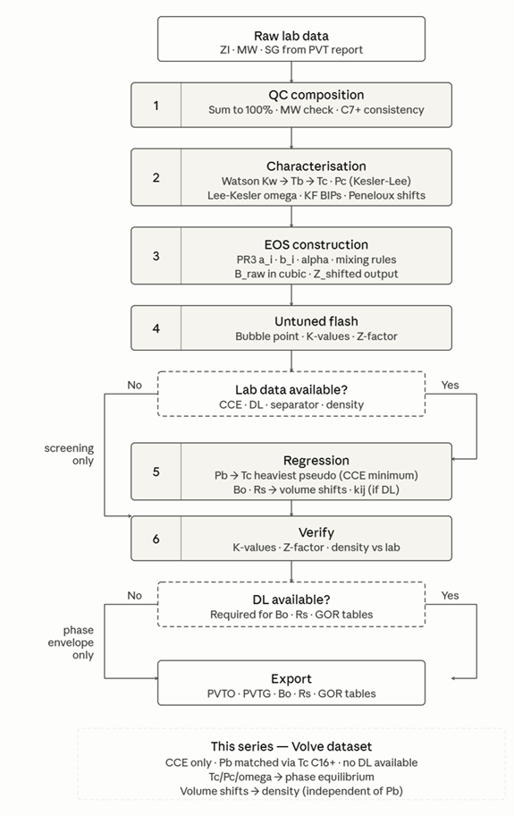
The workflow below summarises the full characterisation and EOS matching process. CCE is the minimum laboratory requirement — it gives the bubble point and is sufficient to tune the EOS for phase equilibrium. Differential liberation extends the regression to volumetric properties and enables Eclipse keyword export. For the Volve fluid used in this series only CCE data was available. The workflow stops at bubble point verification.
Data and Code
Full Jupyter notebooks: github.com/eskoantg/PVTi_cross_check
Volve dataset: equinor.com/energy/volve-data-sharing
See Part 1 for data sources and disclaimer.
▶ Nomenclature (click to expand)
| Symbol | Description | Units |
|---|---|---|
| P | Pressure | bar |
| T | Temperature | K |
| Tc | Critical temperature | K |
| Pc | Critical pressure | bar |
| ω | Acentric factor | — |
| F | Regression objective function | bar² |
| Ki | K-value (equilibrium ratio) | — |
| zi | Overall mole fraction | — |
| Amix | Dimensionless mixture attractive parameter | — |
| ai | Pure-component attractive parameter | cm⁶·bar/mol² |
| Pbub | Bubble point pressure | bar |
References
- Peng, D.Y. and Robinson, D.B. (1976). A New Two-Constant Equation of State. Industrial & Engineering Chemistry Fundamentals, 15(1), 59-64.
- Peneloux, A., Rauzy, E. and Freze, R. (1982). A Consistent Correction for Redlich-Kwong-Soave Volumes. Fluid Phase Equilibria, 8, 7-23.
- Kesler, M.G. and Lee, B.I. (1976). Improve Prediction of Enthalpy of Fractions. Hydrocarbon Processing, 55(3), 153-158.
- Whitson, C.H. and Brulé, M.R. (2000). Phase Behavior of Petroleum Reservoir Fluids. SPE Monograph Series.
- Coats, K.H. and Smart, G.T. (1986). Application of a Regression-Based EOS PVT Program to Laboratory Data. SPE Reservoir Engineering, 1(3), 277-299.
- Equinor (2018). Volve Field Data Village. equinor.com/energy/volve-data-sharing